This article is a brief translation of the blog post Nine levels of EM algorithm by Chunqi Shi. In addition, I add some personal explaination and comprehension, along with sections of relevant papers.

It aims at providing an introduction to EM algorithm. In specific, Shi divides his understanding of EM algorithm into 9 "levels".

(If you have any question or doubt about this article, pls contact me @ hanggao1@umbc.edu)

9 "Level" Comprehension of EM Algorithm

EM is E + M
EM iteratively picks a lower bound
K-means clustering is an example of Hard EM
From EM to general EM
VBEM is a special case of general EM
WS algorithm is another special case of general EM
Gibbs Sampling is also a special case of general EM
WS algorithm is a brief version of VAE and GAN combination
The unity of KL divergence

EM algorithm is E expectation + M maximization

(Do. & Batzoglou) gives a classic example about EM algorithm in What is the expectation maximization algorithm?

Consider a simple coin flipping experiment in which we are given a pair of coin A and B of unknown biases, $ \theta_A $ and $ \theta_B $ respectively (i.e., given any flip, coin A will land on heads with probability $\theta_A$ and tails with probability $ 1-\theta_A $ and similar for coin B).

If the goal is set to estimate $\theta = (\theta_A, \theta_B)$, we can divide the experiment into n repeated runs of the following procedure: (1) randomly choose one of the two coins; (2) and perform m independent coin tosses with the selected coin.

In other words, we keep track of two vectors $ x = (x_1, x_2, …, x_n) $ and $ z = (z_1, z_2, …, z_n) $, where $ x_i \in \{0, 1, 2, …, m\} $ is the number of heads observed during the ith set of tosses, and $ z_i \in \{A, B\} $ is the identity of the coin used for ith set of tosses.

In this setting, parameter estimation is known as the complete data case (values of all relevant variables are known), then $ \theta_A $ and $ \theta_B $ can be given as, $ \hat{\theta_A} = \frac{H_A}{H_A + T_A} $ and $ \hat{\theta_B} = \frac{H_B}{H_B + T_B} $, where $ H_A $ is the # of heads using coin A and $ T_A $ is the # of tails using coin A and similiar for B.

Fig 1: Parameter estimation for complete and incomplete data

The above estimation is known as maximum likelihood estimation in statistical literature, i.e., it gives a solution of the parameters $ \hat{\theta} = (\hat{\theta_A}, \hat{\theta_B}) $ that maximize the logarithm of joint probability (or log-likelihood) $ log p(x, z; \theta) $.

However, when it comes to incomplete data case, for example, we are only given recorded head counts $ x $, without the identities $ z $ of the coin used for each set of tosses. In this case, it is impossible to compute the propotion of heads for each coin because coin identity is no longer available. However, viewing $z$ as latent factors or hidden variables, if we have some way to complete data, we can reduce the problem of parameter estimation with incomplete data back to maximum likelihood estimation with complete data.

One possible completion could be as follows: (1) starting from some initial parameters, $\hat{\theta}^t = (\hat{\theta_A}^t, \hat{\theta_B}^t)$, determine for each run whether coin A or B was more likely to have generated the observed flips (using current parameter estimates); (2) assume the guess/completetion to be correct (coin assignment), apply regular maximum likelihood estimation to get $\hat{\theta}^{t+1}$; (3) repeat the above two steps until convergence. The completion will improve along with the improvement of parameter estimates.

Expectation maximization is a refinement on the above idea. Instead of picking the most possible coin for each run on each iteration, EM computes probabilities for each completion of missing data, using current parameters $\hat{\theta}^t$. A weighted training data is thus created consisting of all possible completion of data. And then a modified version of maximum likelihood estimation deals with the weighted training examples and provides new parameter estimates $ \hat{\theta}^{t+1} $. By using weighted training examples rather than choosing the single best completion, EM is able to account for the confidence of the model in each possible completion.

Back to the definition that EM is E + M, expectation maximization alternates between E and M step. At E step, EM tries to approximate a probability distribution over completions of missing data given current model while at M step, EM re-estimates the model parameters using these completions. However, it is often not necessary to compute the probability distribution over completions, instead, "expected" sufficient statistics is enough,

\[ Q(\theta|\theta^t) = E_{z|x,\theta^t}(log L(\theta; x, z)) \]

where $ L(\theta; x, z) = p(x, z|\theta) $ is the likelihood function, and model reestimation can be thought as maximization of the expected log likelihood of completed data.

\[ \theta^{t+1} = \underset{\theta}{\operatorname{argmax}} Q(\theta|\theta^t) \]

EM iteratively picks a lower bound

Above we provide the explaination of EM on finding the parameters $ \hat{\theta} $ that maximizes log-probability $ log p(x; \theta) $. Generally speaking, the optimization problem addressed by EM is more difficult than the optimization used in maximum likelihood estimation. That is, in the complete data case, $ log p(x, z; \theta) $ has a single global optimum, which can often be found in closed form with maximum likelihood optimization, while for incomplete data case, $ log p(x; \theta) $ has multiple local maxima and usually no closed form solutions.

EM solves the issue by reducing the problem of optimizing $ logp(x; \theta) $ into a sequence of simpler optimization subproblems, whose objective functions have unique global optima that can often be computed in closed form. These problems are chosen in a way that gaurantees their solutions $ \hat{\theta^1} $, $ \hat{\theta^2} $ … and will converge to local optimum of $ log p(x; \theta) $

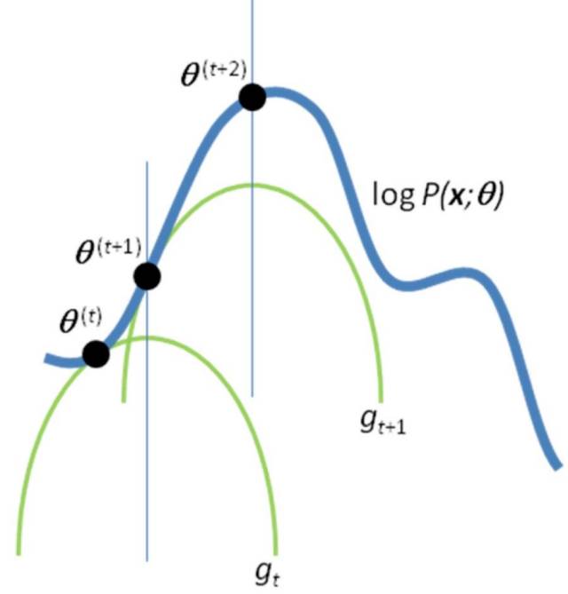
In fact, with Jensen Inequality, we can get a lower bound of $ logp(x; \theta) $,

$\begin{align} logp(x | \theta) & = log(\int p(x, z | \theta) dz) = log(\int q(z)\frac{p(x, z | \theta)}{q(z)} dz) \\ & = log E_q[\frac{p(x, z | \theta)}{q(z)}] = log E_q[e^{log\frac{p(x, z | \theta)}{q(z)}}] \\ & \ge log e^{E_q[log\frac{p(x, z | \theta)}{q(z)}]} \\ & \ge E_q[log\frac{p(x, z | \theta)}{q(z)}] \\ \end{align}$

where $ q $ is an arbitrary distribution for missing data variable $ z $.

Remark. For some paticular $ \theta^t $, the above inequality holds with equality if $ q(z) = p(z | x, \theta^t) $.

Proof. Let $ L(\theta^t; q) = E_q[log\frac{p(x, z | \theta^t)}{q(z)}] $, if $ q(z) = p(z | x, \theta^t) $, we have,

$\begin{align} L(\theta^t; q) &= E_q[log\frac{p(x, z | \theta)}{q(z)}] \\ &= \int p(z|x, \theta^t)[log\frac{p(x, z | \theta)}{p(z|x, \theta^t)}] dz\\ &= \int p(z|x, \theta^t)[log\frac{p(z|x, \theta^t)p(x|\theta^t)}{p(z|x, \theta^t)}] dz \\ &= \int p(z|x, \theta^t) log p(x|\theta^t) dz \\ &= log p(x |\theta^t) \int p(z|x, \theta^t) dz \\ &= log p(x |\theta^t) \end{align}$

Recall that we mentioned above that E step aims at guessing the probability distribution of completions given current model, which in other words, is to pick the right $ q(z) $ for the lower bound here. In order to achieve faster optimization, we usually pick a $ q(z) $ that provides the tightest bound, i.e., at E step, for iteration t, we assign a value to $ q^{t+1} $, so that,

$\begin{align} q^{t+1} &= \underset{q}{\operatorname{argmax}} L(\theta^t; q) \\ &= p(z|x, \theta^t) \end{align}$

Then at M step, we update parameter $ \theta $ with $ \theta^{t+1} $ that maximizes the lower bound above,

$\theta^{t+1} = \underset{\theta}{\operatorname{argmax}} L(\theta; q^{t+1})$

In this way, we have $ logp(x;\theta^t) = L(\theta^t; q^t) \le L(\theta^t; q^{t+1}) \le L(\theta^{t+1}; q^{t+1}) = logp(x; \theta^{t+1}) $, i.e., the objective function monotonically increases for each iteration, and eventually it will converge to some local optimum as with most optimization methods for nonconcave functions.

Fig 2: A sequence of optimization subproblems. g is the lower bound function for each iteration. Note black circle means the point where the tightest bound is obtained.

K-means clustering is an example of Hard EM

Recall above we talked about EM algorithm on maximizing incomplete data log-likelihood $ logp(x; \theta) $, now let’s move to the case of clustering, i.e., given a set of input observations $x_1, x_2, …, x_n$ and only this information, assign cluster/class labels $z_1, z_2, …, z_n$ to each of them.

Hard EM

Let $ \Theta $ be the model parameters, given the problem above, hard EM approximately solves the following optimization problem:

$\Theta^* = \underset{\Theta}{\operatorname{argmax}}\underset{z_1, z_2, ..., z_n}{\operatorname{max}} P_{\Theta}(x_1, x_2, ..., x_n, z_1, z_2, ..., z_n)$

A local optimum of this problem can be found by coordinate ascent, where the coordinates can be defined as coordinate $ \Theta $ and coordinate $ (z_1, z_2, …, z_n) $. Hard EM thus alternatively "ascent" each coordinate with the following procedure in order to maximize $ P_{\Theta}(x_1, x_2, …, x_n, z_1, z_2, …, z_n) $

Initialize $ \Theta $
Repeat until convergence of $ P_{\Theta}(x_1, x_2, …, x_n, z_1, z_2, …, z_n) $
1. $ (z_1, z_2, …, z_n) := \underset{z_1, z_2, …, z_n}{\operatorname{argmax}} P_{\Theta}(x_1, x_2, …, x_n, z_1, z_2, …, z_n) $
2. $ \Theta := \underset{\Theta}{\operatorname{argmax}} P_{\Theta}(x_1, x_2, …, x_n, z_1, z_2, …, z_n) $

K-Means clustering as an example of Hard EM

In K-means, we have $ x_t \in R^D $ and $ z_t \in \{1, 2, …, K\} $. We can define a K-means probability model $ N(\mu, I) $, which is a Gaussian distribution with mean $ \mu \in R^D $ and identity covariance matrix. Then we have,

$\Theta = (\mu^1, \mu^2, ..., \mu^K), \mu^k \in R^D$ $\begin{align} P_{\Theta}(x_1, x_2, ..., x_n, z_1, z_2, ..., z_n) &= \prod_{t=1}^N P_{\Theta}(x_t, z_t) \\ &= \prod_{t=1}^N P_{\Theta}(x_t | z_t)P_{\Theta}(z_t) \\ &= \prod_{t=1}^N \frac{1}{K}N(\mu^{z_t}, I)(x_t) \end{align}$

Let’s reconsider the optimization procedure of hard EM mentioned above. After intitializing parameters, hard EM alternates itertaively between two steps: (1) find assignment of latent varibles $ z_t $ that maximizes the likelihood; (2) find the parameters $ \Theta $ that maximize the likelihood with the assignment obtained at step (1).

In the case of K-means, similarly, after each cluster $ z $ is assigned with a center $ \mu^z $, we repeat the following two steps: (1) decide $ z_t $ for each $ x_t $ given $ (\mu^1, \mu^2, …, \mu^K) $, i.e, find $ z_t $ so that $ x_t $ is closest to $ \mu^{z_t} $; (2) recompute $ \mu^1, \mu^2, …, \mu^K $ given the assignment of $ z_t $ of each $ x_t $. Given the pdf of Gaussian, one can easily show that it is equivalent to the following,

$(\mu^1, \mu^2, ..., \mu^K)^* = \underset{\mu^1, \mu^2, ..., \mu^K}{\operatorname{argmin}} \underset{z_1, z_2, ..., z_n}{\operatorname{min}} \sum_{t=1}^N ||\mu^{z_t} - x_t||^2$

K-Means Clustering as an Example of Hard EM provides a detailed optimization algorithm for K-means in this setting.

Hard vs Soft

CITATIONS:

Fig 1: (Do. & Batzoglou) What is the expectation maximization algorithm?
Andrew Ng. The EM algorithm

Hang Gao

a Ph.D student interested in deep learning